The main point:

Extraneous ARPES data can be exploited to determine experimental unknowns such as inner potential and sample orientation.

Introduction

The momentum of electrons probed by ARPES is related to the observed emission angle and kinetic energy by: $$ E_K = h\nu - \phi - E_B $$ $$ k_\parallel = \frac{1}{\hbar} \sqrt{2 m_e E_K} \sin(\theta) $$ $$ k_\perp = \frac{1}{\hbar} \sqrt{2 m_e (E_K \cos^2 \theta + V_0)} \cos(\theta) $$ The uncertainty in the parallel momentum is dominated by the uncertainty in observed angle (typically $0.1^\circ$). $$ \Delta k_\parallel = \frac{1}{\hbar} \sqrt{2 m_e E_K} \cos(\theta) \Delta \theta $$ The uncertainty in the perpendicular momentum is dominated by the finite probing depth due to the small IMFP of the emitted electrons $$ \Delta k_\perp = \frac{1}{\lambda_{\text{IMFP}}} $$

Methods

We utilize the periodic symmetry of the crystal momentum space to quantitatively compare distinct ARPES measurements whose probed momenta are co-located in the Brillouin zone. A brief description of the algorithm is:

1. Calculate absolute momenta probed by the experiment

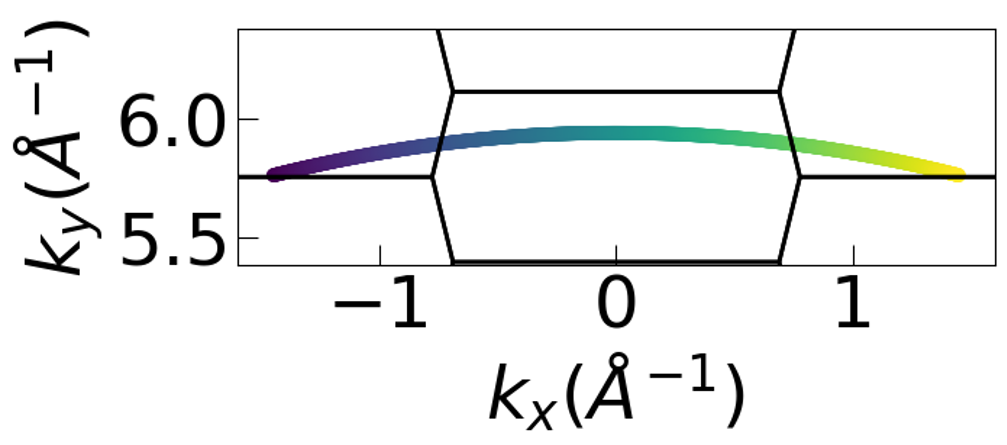
Figure 1 is a visualization of the absolute momenta probed using a 124eV photon energy with a $\pm 15^\circ$ acceptance angle (colorscale is angle of emission) ARPES experiment assuming a work function of 4.5eV and inner potential of 15eV. The Brillouin zone (BZ) of LaNiGa$_2$ is shown in black.

2. Project probed momenta into the 1st Brillouin zone

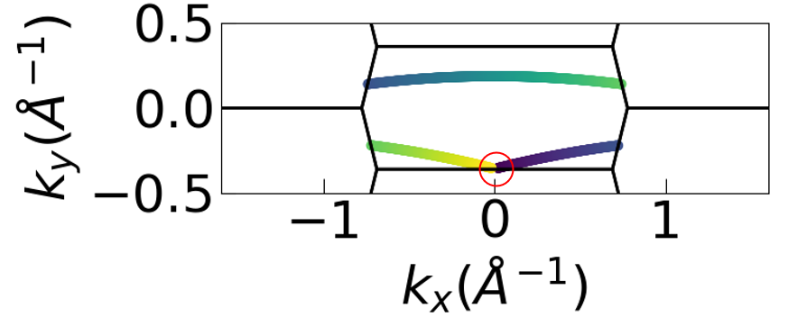
Figure 2 is representing the same momenta of Figure 1 but showing the momenta projected into the 1st BZ. Circled in red is are co-located momenta which originate from very different probed absolute momenta but are equivalent in the BZ.

3. Determine co-located measurements

4. Compare co-located energy distribution curves (EDCs)

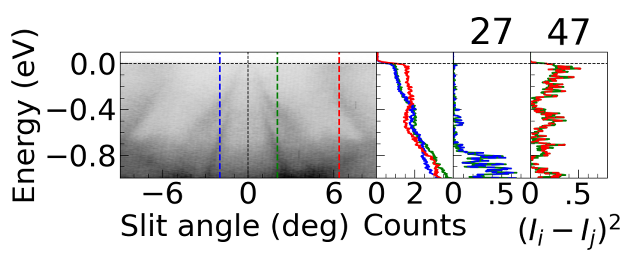
Figure 3 shows the a schematic representation of comparing co-located energy distribution curves (EDCs). Left is an ARPES spectrum with equivalent momenta indicated in blue and green while a non-equivalent momentum is shown in red. The second panel shows the EDCs that are highlighted on the spectrum. It is visually apparent that the blue and green are similar while the red is distinct. The right two panels show the blue and green EDCs subtracted and squared and the red and green respectively. The stronger disagreement of the non co-located EDCs is the foundation for this method.

5. Compute the mean sum-squared-difference of all co-located EDCs ”$\mathcal{D}$” and optimize over parameters like inner potential or sample orientation.

Determining the Inner Potential

By projecting ARPES data from a range of photon energies into the 1st Brillouin zone and comparing co-located EDCs, we get a quantitative handle on the optimal value for the Inner potential.

As an initial test of this method, three datasets have been used:

1. LaNiGa$_2$ platelets cleaved on the platelet face ($b$ axis perpendicular). In the photon energy range of 110eV - 144eV 18 datasets were collected.

2. LaNiGa$_2$ platelets were cleaved along their thin-edge ($a$ axis perpendicular) and in the range of 116eV - 144eV 5 datasets were collected.

3. CeCoGe$_3$ platelets were cleaved and 25 datasets were collected in a photon energy range of 22eV - 118eV.

The common ways of determining the inner potential from ARPES are the following:

1. Observed periodicity over large photon energy range

2. Compare ARPES with calculated band structure

3. Guess? (15eV is usually reasonably close)

The goal of this project is to provide a data-driven alternative that improves on these current methods.

Here, I visualize the effect of a 15eV vs a 5eV inner potential has on the normally cleaved LaNiGa$_2$ dataset.

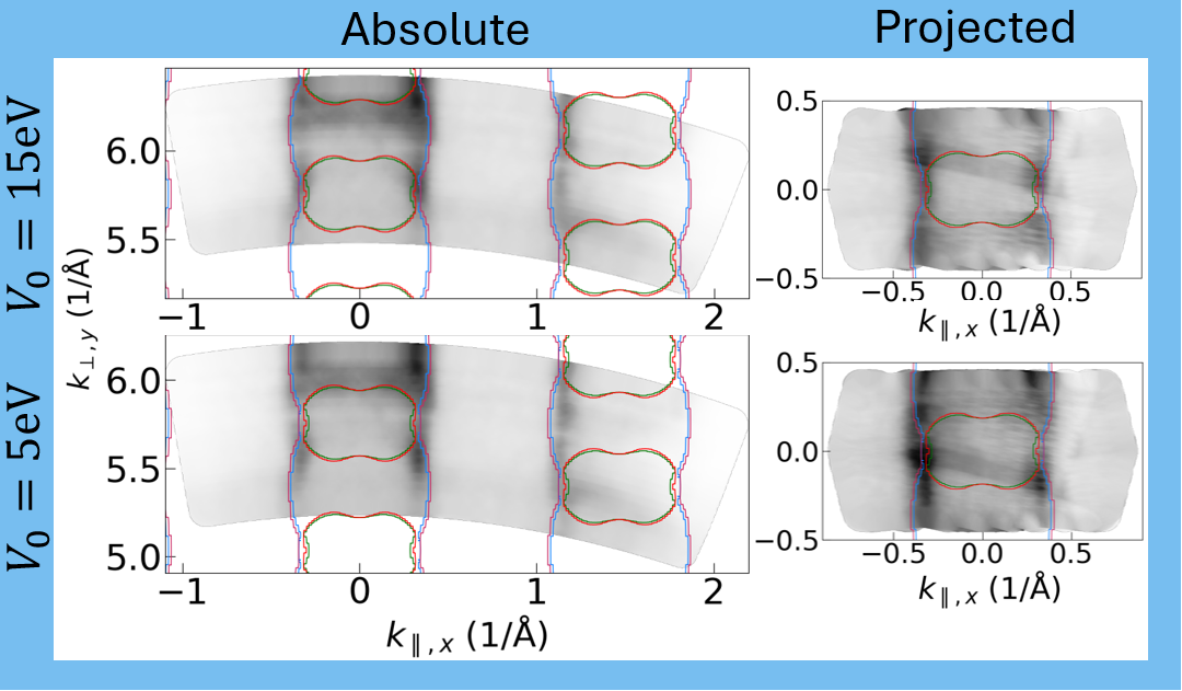
Above, you can see on the left the Fermi surface as a function of perpendicular momentum. Due to the small range of photon energies collected it is not possible to oberserve many periods of the BZ. Instead, we origionally resorted to comparing to the calculated band structure which is overlaid with colored lines.

When inspecting small differences, one can determine that 15eV is a better fit to the calculations than 5eV. However, when trying to determine between 13eV and 15eV for example it would be nearly impossible to tell by eye.

On the right, The data is projected into the 1st BZ and nearly co-located EDCs are integrated to form an “integrated” Fermi surface reconstruction. Here, it is more clear that the 15eV reconstruction “agrees” better in a self-consistent manner. This self-agreement is the basis of the quantitative comparison being used. In addition, the 15eV projection agrees better with the calculated electronic structure.

Using the quantitative measure outlined in the methods, the “Disagreement” ($\mathcal{D}$) is calculated as a funciton of inner potential for all three datasets:

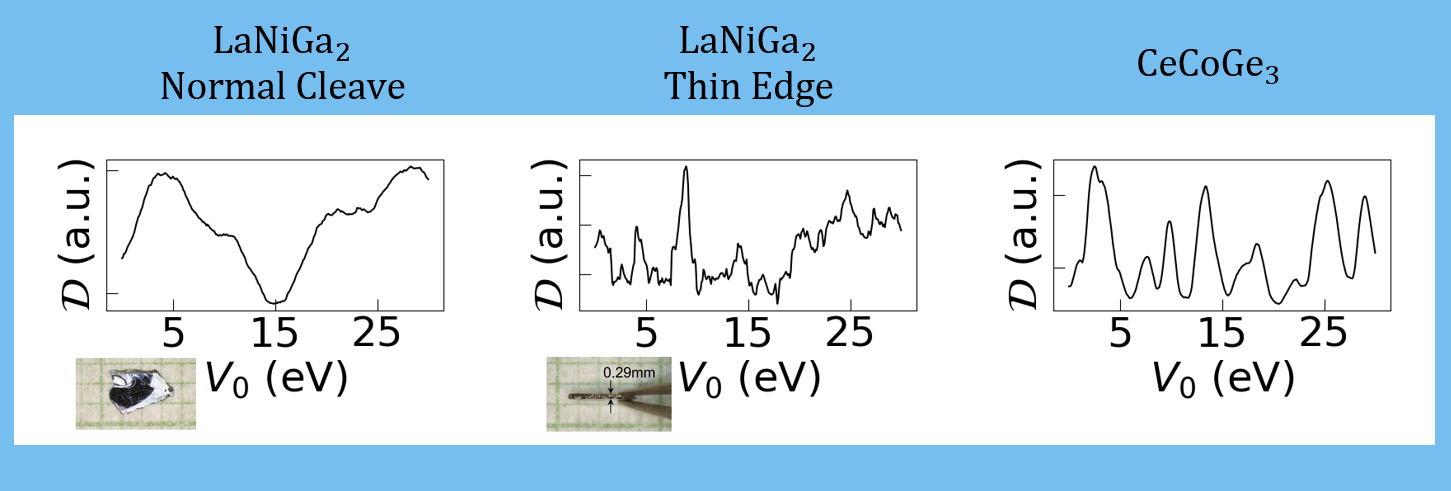
With the normal cleave LaNiGa$_2$, a clear minimum is found at 15eV. For the cases of the thin-edge cleave and CeCoGe$_3$ there are many multiple minima which are more difficult to interpret. For the thin-edge we hypothesize this is due to the small range of photon energies used in combination with the low quality of some of those datasets. In the case of CeCoGe$_3$ we are actively working to understand the multiple minima. Some possibilities include possible additional band folding in the data, noise in the data, and background effects.

Determining sample orientation

In addition to the inner potential, this method can be used to determine the self-agreement of the data as a funciton of any experimetnal unknown.

Here, we explore the dependence on the orientaion of the dataset. The use-case is when exploring novel three-dimensional materials sometimes it can be difficult to determine which orientation your data is being colected due to matrix element effects.

Below, we compare the dependnece of $\mathcal{D}$ as a funciton of orientation angle by rotating the presumed sample normal and slit directions around the $(1,1,1)$ direction by an angle from the known correct orientation.

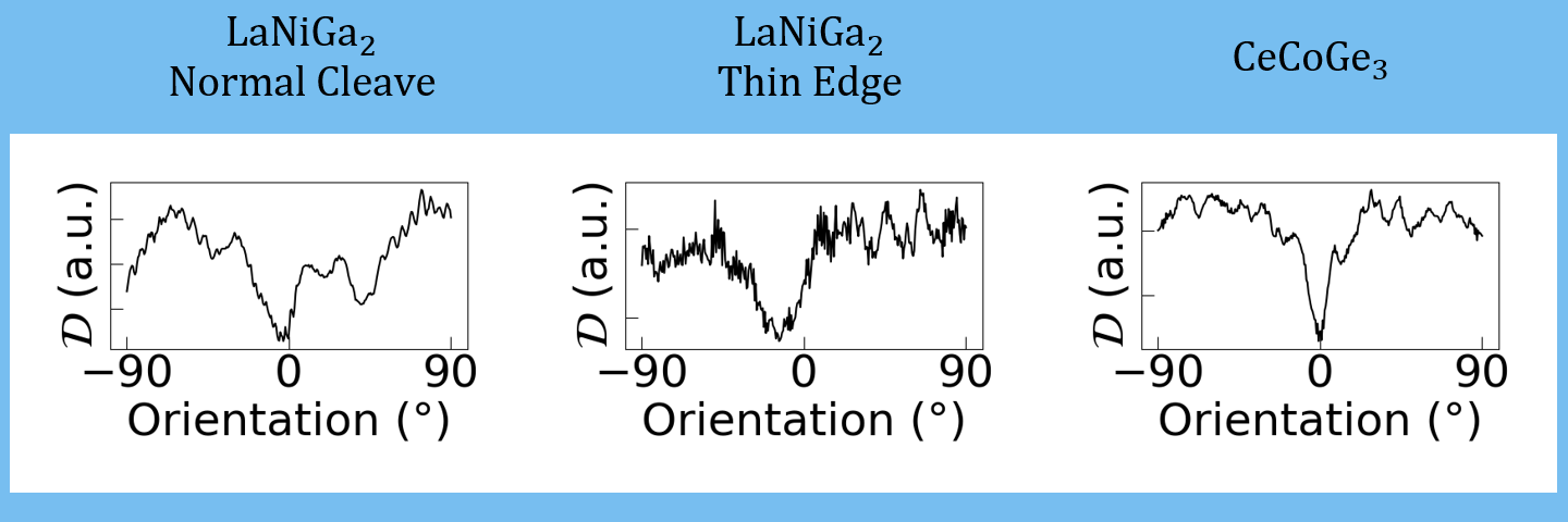
In the orientation a clear minimum is observed for all three datasets near the known orientaion. The thin-edge cleave minimum is offset slightly which may indicate that our dataset was not collected exactly in the orientation we presumed!

The Fermi surface can also be reconstructed as a function of orientation angle, which is performed below. Here we see a striking difference between the apparent symmetry of the correct orientation in contrast to the $5^\circ$ orientation.

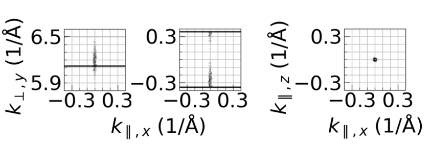
Simulated ARPES by careful consideration of $\Delta k_\perp$

In order to provide a large testbed for this technique, we are developing a method of simulating ARPES data from calculated electronic structure.

The important innovation in this simulation is a careful consideration of the broadening effects in collected ARPES data.

Due to the finite probing depth of ARPES and the uncertainty principle typical ARPES experiments can have a $\Delta k_\perp \approx 0.1 \text{\AA}^{-1}$ which is a significant ($\approx 10%$) portion of the BZ.

Sampling the calculated electronic structure at many points according to both the in-plane and out-of-plane broadening we can account for much of the broadening seen in ARPES data wihout the need of computationally expensive methods like many one-step-model treatments.

Below is an example indicating a sampling of the uncertainty of a single probed momentum both in an absolute momentum (left) and projected (middle) into the 1st BZ. On the right is the in-plane uncertainty.